Introduction

In my Ph.D., one of my projects introduced me to empirical Bayesian methods, in a very simplified setting (using Metropolis-Hastings as the algorithm). However, I’ve become more interested in Bayesian methods recently, and have been trying to use Stan for more analyses. If you’ve ever used Stan, you’re familiar with how challenging the debugging workflow can be with more complex models, so I wanted to focus on something a little easier that I could check easily. One such example is ridge regression, which inspired the work below.

Ridge Regression

One of the commonly-taught techniques for students learning Machine Learning techniques are Ridge and LASSO regression, which are similar to the linear regression techniques with which students are often familiar, while introducing regularization to combat overfitting. Beginning with OLS, the OLS coefficient vector is computed using feature observations \(x_1,...,x_n\) (where each \(x\) observation is \(k\)-dimensional) and corresponding outcomes \(y_1,...,y_n\)

\[ \min_{\hat{\beta}} \quad \sum_{i=1}^n(y_i-x_i^{\top}\hat{\beta})^2 \]

That is to say, the solution minimizes the sum of squared errors. We can then use the coefficient vector \(\beta\) to make predictions on a new observation \(\widetilde{x}\) as

\[ \widetilde{y} = \widetilde{x}^{\top}\hat{\beta} \]

However, in settings where the dimensionality of the observations is large and the data is not (big \(k\) and relatively small \(n\)), the OLS predictions are likely to overfit, so we introduce regularization and (in the Ridge case) solve the problem

\[ \min_{\hat{\beta}} \quad \sum_{i=1}^n(y_i-x_i^{\top}\hat{\beta})^2 + \lambda\;\hat{\beta}^{\top}\hat{\beta} \]

The penalty for larger values of the coefficient vector \(\hat{\beta}\) ensures that overfitting is mitigated, with the degree to which the coefficients are penalized dictated by the hyperparameter of \(\lambda\).

A nice property of Ridge (as opposed to LASSO) is that we get a closed-form solution for the coefficient vector that solves this problem:

\[ \beta_{Ridge} = \left(X^{\top}X + \lambda I\right)^{-1}X^{\top}y \]

We see that this looks very similar to the OLS estimator, but with the additional “denominator” penalty ensuring that the coefficients are generally smaller¹.

Bayesian Regression

One nice thing about Bayesian models is that we can put priors on parameters, and in the case of Bayesian regression, if we pick the right priors, we see that we recover the Ridge regression coefficients exactly. This is part of a broader thing that I find convenient about Bayesian modeling – tight priors around zero enforce a measure of regularization on the model. In particular, if we structure our model to be

\[ y_i = x_i^{\top}\beta + \varepsilon, \quad \varepsilon \sim \mathcal{N}(0, \sigma^2) \]

and we stipulate prior distributions of the form

\[ \begin{split} \sigma &\sim IG(a_0,b_0)\\ \beta|\sigma &\sim \mathcal{N}\left(0, \frac{\sigma^2}{\lambda}I\right)\\ \end{split} \]

then the posterior mean of the coefficient vector will be exactly the Ridge coefficients. Intuitively, as \(\lambda\) (our Ridge penalty) increases, the prior distribution tightens around zero for \(\beta\), and we get more regularization.

Model Assessment

It’s worth saying off the bat: this is a contrived and unnecessary exercise. With our choice of priors above, we get closed-form solutions for the distribution of \(\hat{\beta}\), so sampling is superfluous. However, as I said before, Stan is not particularly intuitive for me, so working through a basic example helped me quite a bit.

We begin by importing an arbitrary dataset, in this case MLB’s Statcast data on pitches thrown in July 2022 via the baseballr package.

suppressPackageStartupMessages({
  library(rstan)
  library(tidyverse)
})

set.seed(18)

sc_raw <- "https://github.com/sportsdataverse/baseballr-data/raw/refs/heads/main/statcast/2022-July-StatcastData.rds" %>%
    read_rds()

We’re going to make predictions about the exit velocity (launch_speed) for a random subset of the balls hit in play. We’ll use a large set of features to mimic a setting where we’d want to add regularization to the problem.

sc_analysis <- sc_raw %>%
  select(
    launch_speed,
    vx0, vy0,
    pfx_x, pfx_z,
    plate_x, plate_z,
    pitch_type, p_throws, balls, strikes, outs_when_up,
    on_3b, on_2b, on_1b,
    release_speed, release_spin_rate,
    pitch_number, platoon_advantage, pitcher_pitch_count, pitcher_ab_count, batter_ab_count
  ) %>%
  # remove infrequent pitch types and balls not hit in play
  filter(!is.na(launch_speed), pitch_type %in% c("CS", "EP", "KN", "FA") == FALSE) %>%
  # convert variables to factor and indicators
  mutate(
    across(c(strikes, balls, outs_when_up), factor),
    across(c(on_1b, on_2b, on_3b), ~ ifelse(is.na(.), 0, 1))
  ) %>%
  # remove observations with missing data
  na.omit()

We’ll create a train and test dataset, both with a (mutually exclusive) random 10% sample of the data².

train_data <- sc_analysis %>%
    slice_sample(prop = .1)

test_data <- sc_analysis %>%
    anti_join(train_data, by = colnames(train_data)) %>%
    slice_sample(prop = .1/.9)

We now create the relevant matrices from the data:

model <- 'launch_speed ~ .'
X <- model.matrix(formula(model), data = train_data)
y <- train_data$launch_speed

X_test <- model.matrix(formula(model), data = test_data)

We can inspect the train and test matrices:

dim(X)

## [1] 3777   32

dim(X_test)

## [1] 3778   32

We can now compute the Ridge coefficients directly and compare them visually:

compute_ridge <- function(lambda, X, y){
  solve(t(X) %*% X + lambda * diag(dim(X)[2])) %*% (t(X) %*% y)
}

less_penalty <- compute_ridge(25, X, y)
more_penalty <- compute_ridge(100, X, y)

tibble(
  less_penalty,
  more_penalty
) %>%
  ggplot(data = .) +
  geom_point(aes(x = abs(less_penalty), y = abs(more_penalty))) +
  geom_abline(linetype = "dashed", color = "darkgreen") +
  labs(x = 'Ridge Coefficient Magnitude (Lambda=25)',
       y = 'Ridge Coefficient Magnitude (Lambda=100)') +
  theme_bw()

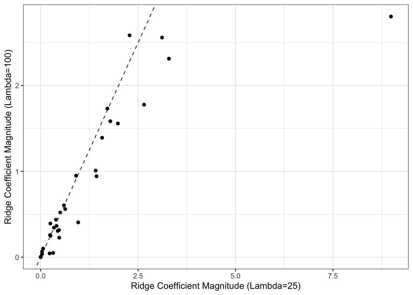
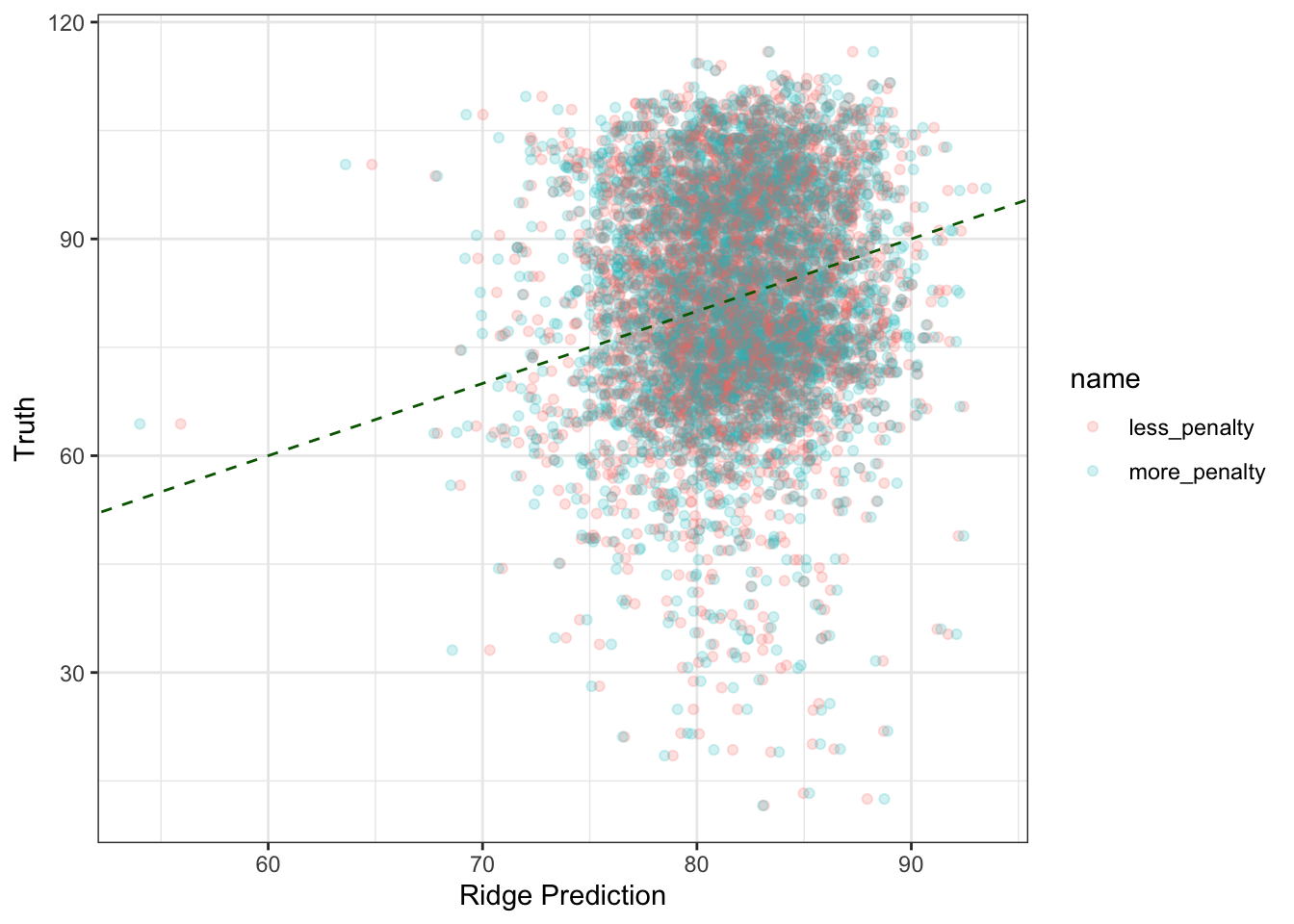
We see that generally (but not always) the coefficients are larger (to the right of the green 45-degree line) when the penalty is smaller – this makes sense, as this model is subject to less regularization. We can also compare out of sample predictions:

ridge_predictions <- tibble(
  'less_penalty' = X_test %*% less_penalty,
  'more_penalty' = X_test %*% more_penalty,
  'truth' = test_data$launch_speed
) 

ridge_predictions %>%
  pivot_longer(c('less_penalty', 'more_penalty')) %>% 
  ggplot(data = .) +
  geom_point(aes(x = value, y = truth, color = name), alpha = .2) +
  geom_abline(linetype = "dashed", color = "darkgreen") +
  labs(x = 'Ridge Prediction',
       y = 'Truth') +
  theme_bw()

We can also of course just compute the MSE between the two models:

mean((ridge_predictions$more_penalty - ridge_predictions$truth)^2)

## [1] 238.8288

mean((ridge_predictions$less_penalty - ridge_predictions$truth)^2)

## [1] 238.0886

So the model with \(\lambda=25\) appears to do better. Can we replicate these findings using stan?

rstan Implementation

We begin by defining the model outlined in the Bayesian Regression section:

stan_code <- "
data {
    int n;
    int k;
    int n_test;
    vector[n] y;
    matrix[n,k] X;
    matrix[n_test,k] X_test;
    real<lower=0> lambda; // the amount of regularization in the model
}
parameters {
    real<lower=0> sigma;
    vector[k] beta;
}
model {
    sigma ~ inv_gamma(100,100);
    beta ~ normal(0, sigma/lambda);
    target += normal_lpdf(y - X*beta | 0, sigma);
}
generated quantities {
    vector[n_test] y_pred;
    for (i in 1:n_test)
        y_pred[i] = normal_rng(X_test[i] * beta, sigma);
}
"

As we’re specifying the standard deviation within Stan as opposed to the variance, we have to pass in \(\lambda\)’s square root when we call the models:

fit_less_reg <- stan(
    model_code = stan_code,
    data = list(
        n = nrow(X),
        k = ncol(X),
        n_test = nrow(X_test),
        y = y,
        X = X,
        X_test = X_test,
        lambda = sqrt(25)
    ),
    chains = 4,
    warmup = 1000,
    iter = 8000,
    cores = 4,
    control = list('max_treedepth' = 20)
)

fit_more_reg <- stan(
    model_code = stan_code,
    data = list(
        n = nrow(X),
        k = ncol(X),
        n_test = nrow(X_test),
        y = y,
        X = X,
        X_test = X_test,
        lambda = sqrt(100)
    ),
    chains = 4,
    warmup = 1000,
    iter = 8000,
    cores = 4,
    control = list('max_treedepth' = 20)
)

A few notes on the above:

• I manually increased the max_treedepth parameter because of how often the default limit of 10 was being hit; Stan’s documentation suggests that this is more of a computational/efficiency concern as opposed to a model concern.
• We’re sampling quite a few times – this is because the Effective Sample Size (ESS) winds up being relatively small, so we need many draws to have confidence that we’re getting a good representation of the posterior. This is particularly important for smaller values of \(\lambda\), where the prior is less informative.

We can now inspect the results:

post_means <- bind_rows(
  fit_less_reg %>% 
    get_posterior_mean() %>% 
    as_tibble(., rownames = "parameter") %>%
    filter(str_detect(parameter, "y_pred\\[\\d+\\]")) %>%
    select(estimate=`mean-all chains`) %>% 
    mutate(model = 'less_penalty',
           truth = test_data$launch_speed),
  fit_more_reg %>% 
    get_posterior_mean() %>% 
    as_tibble(., rownames = "parameter") %>%
    filter(str_detect(parameter, "y_pred\\[\\d+\\]")) %>%
    select(estimate=`mean-all chains`) %>% 
    mutate(model = 'more_penalty',
           truth = test_data$launch_speed)
)

ggplot(data = post_means) +
  geom_point(aes(x = estimate, y = truth, color = model), alpha = .2) +
  geom_abline(linetype = "dashed", color = "darkgreen") +
  labs(x = 'Ridge Prediction',
       y = 'Truth') +
  theme_bw()

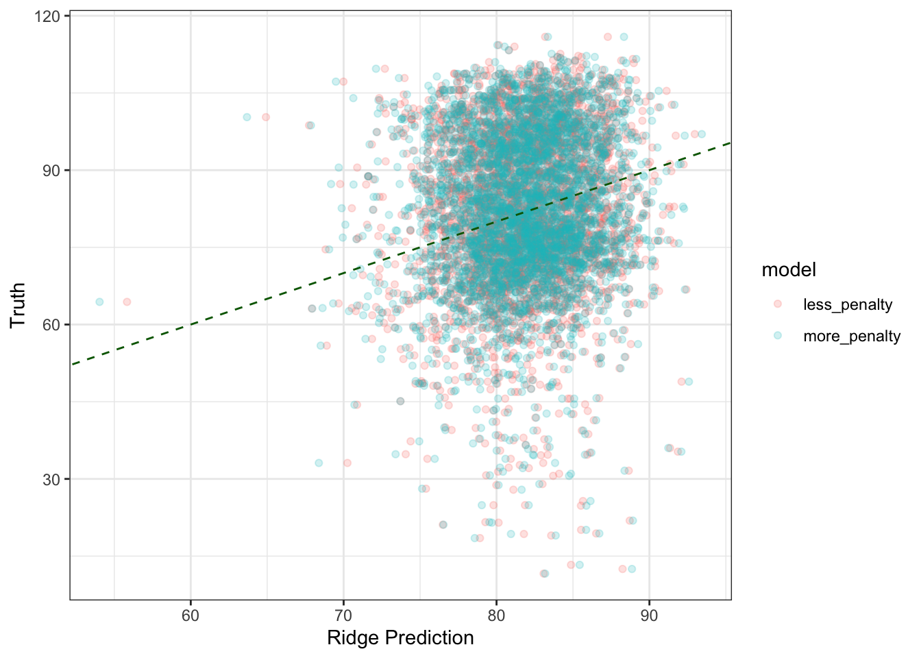
It looks the same! The cool thing about this is that we have samples of the posterior predictive distribution for any given datapoint we’re trying to predict:

less_reg <- as.data.frame(fit_less_reg)
more_reg <- as.data.frame(fit_more_reg)

plot_prediction <- function(idx){
  more <- more_reg %>% pull(str_interp('y_pred[${idx}]'))
  less <- less_reg %>% pull(str_interp('y_pred[${idx}]'))
  ggplot() +
    geom_histogram(aes(x = more), alpha = .1, fill = "blue", bins = 50) +
    geom_histogram(aes(x = less), alpha = .1, fill = "red", bins = 50) +
    geom_vline(
        xintercept = test_data$launch_speed[idx],
        color = "darkgreen",
        linetype = "dashed"
    ) + 
    labs(x = 'Exit Velocity',
         y = 'Simulations') +
    theme_bw()
}

plot_prediction(40)

plot_prediction(300)

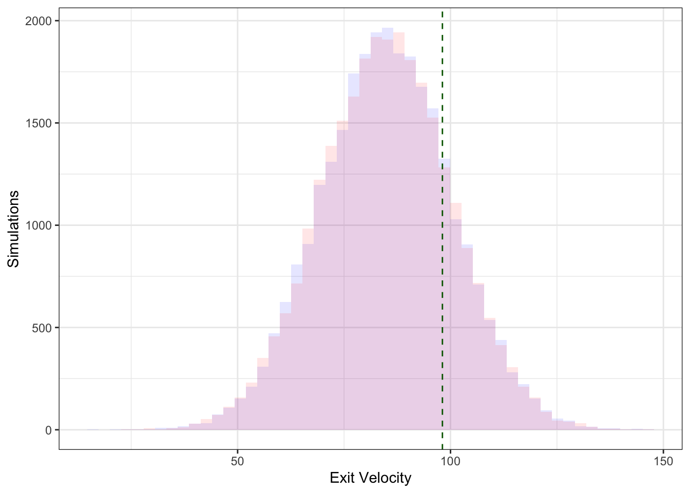
Here, the colors represent the two different models, and the dashed green line represents the actual observed exit velocity – we see the distributions are very similar (as the models are quite similar).

Conclusion

Don’t do this! We have a conjugate prior here, so we don’t need Stan. But if you’re trying to fit a basic Stan model that will require (relatively) little debugging, Ridge is a good choice, and it provides some intuition for how to regularize parameters in Bayesian models.